 is a bi-measurable
  stochastic process on
 ![$ [0,T] $](/sites/default/files/tex/b9baa7710b108fe1c29bd70224f83e1ccc813636.png) , it can be considered as a random variable valued in the Hilbert space
, it can be considered as a random variable valued in the Hilbert space ![$ H = L^2([0,T]) $](/sites/default/files/tex/00877b76d19e19f0137f4e585fcc7210328d864d.png) .
.
In [1], it is shown that in the Gaussian case, if the covariance function  is continuous, linear subspaces
  of
of  spanned by
  -stationary codebooks correspond to principal components of , in other words, are spanned by eigenvectors of the covariance operator of .
Thus, the quantization consists first in exploiting the Karhunen-Loève decomposition. The discretization consists in truncating the decomposition at a fixed order  and to quantize the
  -value Gaussian vector constituted of the first coordinates of the process on its Karhunen-Loève decomposition.
To reach optimal quantization, one has both to determine the optimal rank of truncation (the quantization dimension) and to determine the optimal -dimensional Gaussian quantizer corresponding to the first coordinates.
Formally, if is a bi-measurable ![$ L^2([0,T]) $](/sites/default/files/tex/5dac4e73536ca47ece3e71da86eb09c8f7544b45.png) Gaussian process, with a continuous covariance function, its Karhunen-Loève expansion
Gaussian process, with a continuous covariance function, its Karhunen-Loève expansion  writes:
![$\displaystyle X = \sum\limits_{k=1}^\infty \xi_n^X e_n^X \ \in L^2(\Omega \times [0,T]), $](/sites/default/files/tex/e85101a4db542dddfa6bdadc8e23e77231cdcf15.png)
 is a sequence of independent Gaussian random variables.
The terms of the Karhunen-Loève decomposition are explicit for classical Gaussian processes (the standard Brownian motion, the Brownian bridge and the Ornstein-Uhlenbeck process).
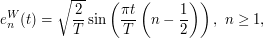
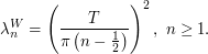
- The Karhunen-Loève decomposition of the standard Brownian motion
 on is:
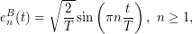
- The Karhunen-Loève decomposition of the standard Brownian bridge
 on is:
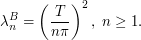
In this case, the -dimensional random vector to be quantized is a Gaussian vector with diagonal variance-covariance matrix  with
with 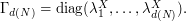
Optimal quantization of the Brownian motion
![]() brownian_optimal_grids.zip
brownian_optimal_grids.zip
The compressed folder brownian_optimal_grids.zip contains optimal quantization grids of the standard Brownian motion.
To get optimal quantization, the point now is to quantize the finite-dimensional Gaussian vector 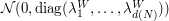 optimally.
Hence, the method is the same as for the standard distribution except that the simulated Gaussian vector is not standard. For a given size , all possible dimensions are tested, and the one that yields the smaller quadratic distortion () is kept.
For a given size  , the text files are organized as follows. It presents in the form of a matrix
  with
with  rows and
  columns.
- On row
 : Element
  of the grid and its companion parameters. Consider
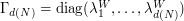
![$$
G_{i,1} = \left(\textrm{weight of the Voronoi cell of element } i \right)= \mathbb{P}[ \mathcal{N}(0,\Gamma_{d(N)}) \in C_i(G) ].
$$](/sites/default/files/tex/5b14e454943caa6f8a85b1a4c489190f14a2a4d7.png)


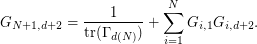
- On last row
 :
:


In particular we can verify that
 |
 |
For further details and further reading, let us refer to [1].
Product quantization of the Brownian motion and the Brownian bridge
An other way to get a good quantizer of a Gaussian process is Product Quantization. In practice, being settled, one determines the truncation threshold of the decomposition and then, is approximated by 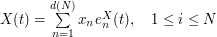 where
where  is a quantizer of the
  -valued random vector
  .
.
The product quantization consists in choosing the quantizer of  as a Cartesian product of one dimensional quantization grids.
Thus, one replaces 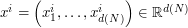 by
by 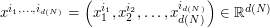 where
where  ,
,  are optimized quantizers of the
  -dimensional Gaussian distribution, of size
  , and where the values are such that
  . A database of optimal quadratic quantizers of the standard Gaussian distribution is available here.
After all, one has for a settled integer to determine among all its possible product decomposition the one that minimizes the distortion error.
In article [2], the optimal product decompositions are used to compute Asian option prices in a stochastic volatility model.
Data to download:
|
|
|
The text file RECORD_QF.TXT contains optimal product decompositions for the standard Brownian motion of size  to
to  .
.
The text file RECORD_QF_BB.TXT contains optimal product decompositions for the standard Brownian bridge of size to .
The both cases two first columns give, for a number  , the value of the distortion of the optimal product quantization.
The following columns give the size  of the best product quantizer for a maximum number of points of , and the corresponding distortion. At least, the corresponding optimal product decomposition is given.
